UK Museums

Data Context

The visualization uses TidyTuesday’s Museums dataset (Nov 2022), whose data context and information can be accessed at this link

museums <- readr::read_csv('https://raw.githubusercontent.com/rfordatascience/tidytuesday/master/data/2022/2022-11-22/museums.csv')

Research Question

Comparing Area Deprivation Indexes Between Large-Sized and Small-to-Medium-Sized Operating Museums in London

Data Transformation

data <- museums %>%
  filter(Size != "unknown") %>%
  filter(Year_closed == "9999:9999") %>% # select museums that are still open
  filter(str_detect(Admin_area, "London")) %>%
  mutate(size_cat = case_when(Size %in% c("huge", "large") ~ "Large",
                              Size %in% c("medium", "small") ~ "Small/Medium")) %>%
  select(Accreditation, size_cat, Size, starts_with("Area_Deprivation_index")) %>%
  rename_with(~ sub("Area_Deprivation_index_", "", .x), starts_with("Area_Deprivation_index_")) 
 

data <- na.omit(data)

Data Visualization

Since there are multiple area deprivation indexes, I decided to create a correlation matrix for the Area Deprivation Indexes in our data to see if there is any highly correlated feature that can be removed.

corrplot(cor(data[5:11]), method = 'color', order = 'FPC', type = "lower", diag = FALSE, col = COL1('Purples'), addCoef.col = 'white', title = "Correlation Matrix of Area Deprivation Indexes", mar=c(0,0,1,0), tl.col="black")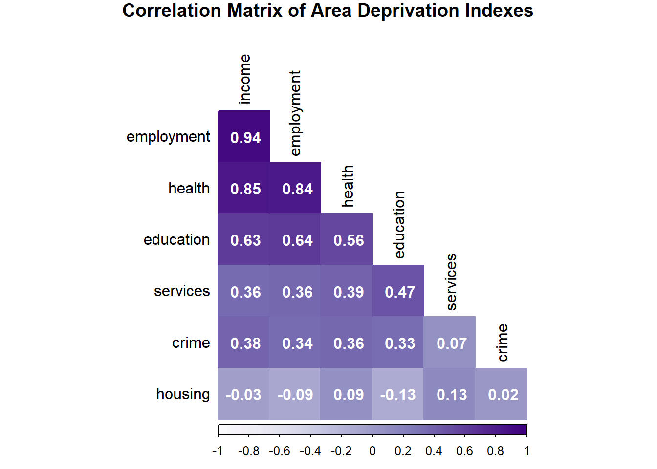

As seen in the plot, the health, income, and employment indexes are highly correlated. Since income is the first variable in the first principal component (FPC), I keep it in the dataset while removing the other two variables for my parallel plot.

showtext_auto()

data %>%
  select(-c(health, employment)) %>%
  ggparcoord(
    columns = 5:9, groupColumn = 2, scale = "globalminmax",
    showPoints = FALSE, 
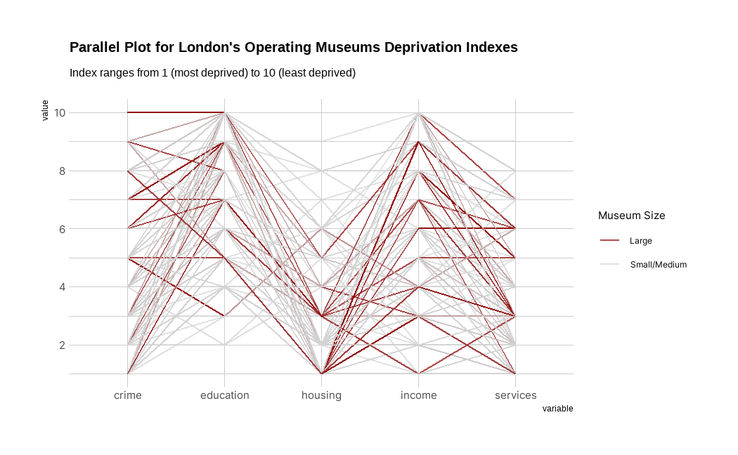
    title = "Parallel Plot for London's Operating Museums Deprivation Indexes",
    alphaLines = 0.7
    ) + 
  scale_y_continuous(breaks = c(0, 2, 4, 6, 8, 10)) +
  scale_color_manual(values = c("darkred", "lightgray")) +
  labs(subtitle = "Index ranges from 1 (most deprived) to 10 (least deprived)",
       color = "Museum Size") +
  theme_ipsum()+
  theme(plot.title = element_text(size=15), 
        text = element_text(family = "Inter"))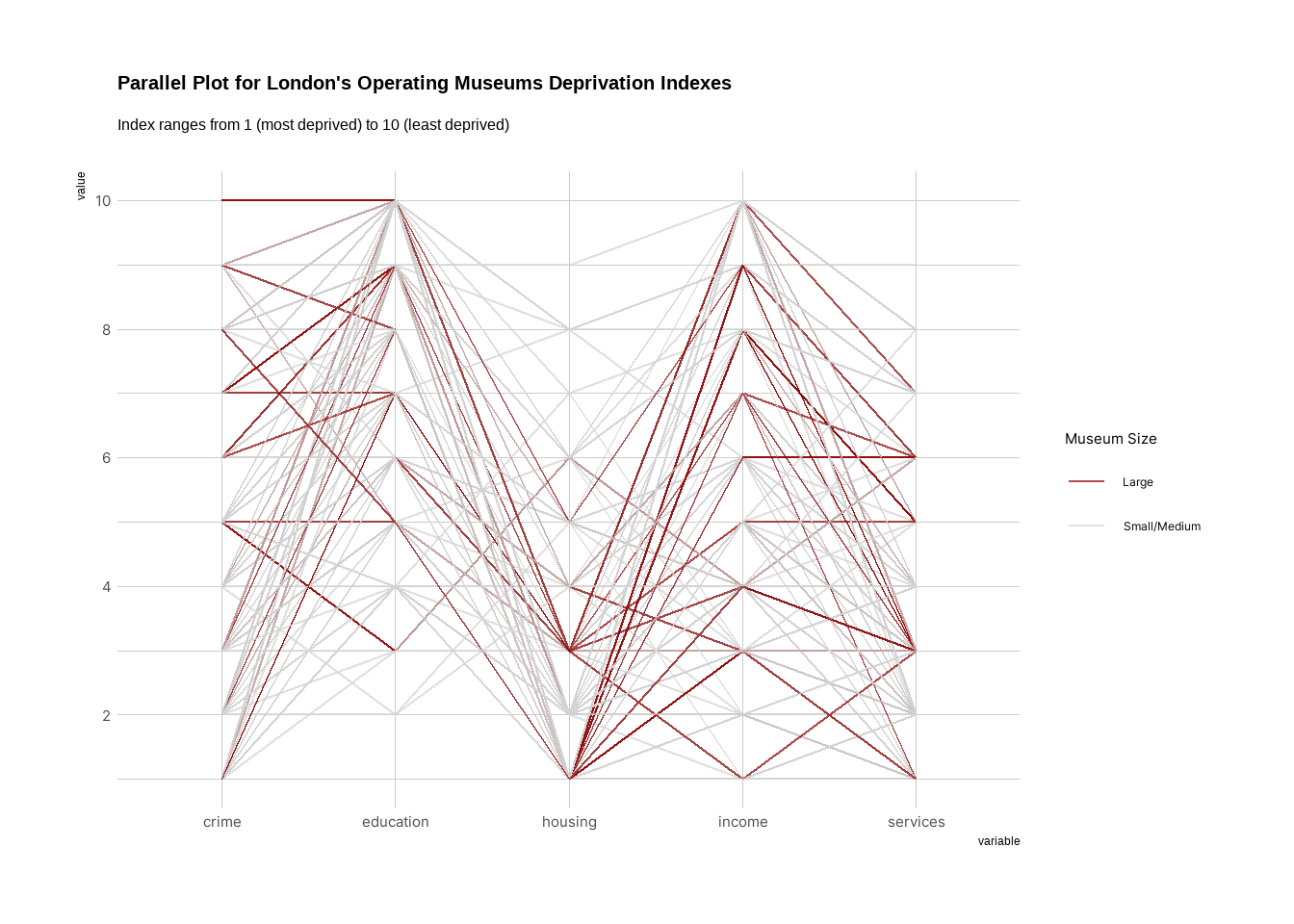

Operating, larger-sized museums in London are more likely to locate in areas with lower housing availability and relatively high education access.