historical_spending <- readr::read_csv('https://raw.githubusercontent.com/rfordatascience/tidytuesday/master/data/2024/2024-02-13/historical_spending.csv')Data Context
The visualization uses TidyTuesday’s Valentine’s Day Consumer Data dataset (Feb 2024), whose data context and information can be accessed at this link
Research Question
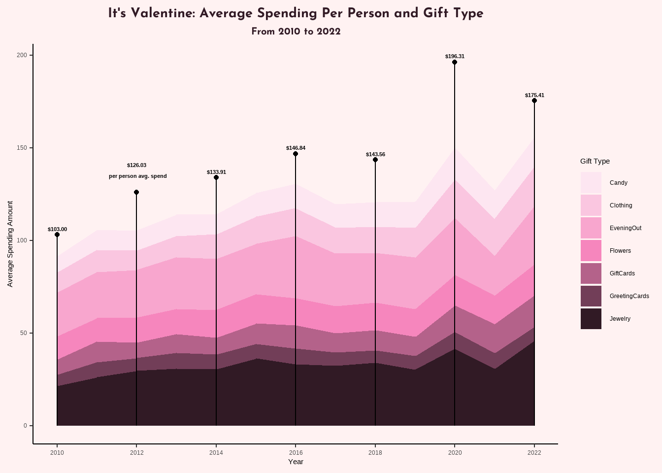
How do Valentine Day’s consumer spending change across the years?
Data Transformation
gifts_year_long <- historical_spending %>%
  select(-c(PercentCelebrating, PerPerson)) %>%
  pivot_longer(cols = !Year, names_to = "gift_type", values_to = "avg_amt")
Data Visualization
Code
showtext_auto()

annot <- function(x_pos, y_pos, label_string) {
  annotate("text", x = x_pos, y = y_pos,
           label = label_string,
           hjust = 0.5, vjust = -1,
           size = 3, lineheight = .8,
           fontface = "bold")
}

style = element_rect(fill = "#fff2f2", color = "#fff2f2")

ggplot(gifts_year_long, aes(x = Year, y = avg_amt)) +
  geom_area(colour = NA, aes(fill = gift_type)) +
  scale_x_continuous(breaks = c(2010,2012,2014,2016,2018,2020,2022), limits = c(2010,2022)) +
  labs(title = "It's Valentine: Average Spending Per Person and Gift Type", subtitle = "From 2010 to 2022", y = "Average Spending Amount", fill = "Gift Type") +
  scale_fill_manual(values = generate_palette("#f686bd",
                             modification = "go_both_ways",
                             n_colours = 7)) +
  #segment
  geom_segment(aes(x = 2010, y = 0, xend = 2010, yend = 103)) +
      geom_point(aes(x = 2010, y = 103.00)) +
      annot(2010, 103.00, "$103.00") +
  geom_segment(aes(x = 2012, y = 0, xend = 2012, yend = 126.03)) +
      geom_point(aes(x = 2012, y = 126.03)) +
      annot(2012, 126.03, "$126.03 \n per person avg. spend") +
  geom_segment(aes(x = 2014, y = 0, xend = 2014, yend = 133.91)) +
      geom_point(aes(x = 2014, y = 133.91)) +
      annot(2014, 133.91, "$133.91") +
  geom_segment(aes(x = 2016, y = 0, xend = 2016, yend = 146.84)) +
      geom_point(aes(x = 2016, y = 146.84)) +
      annot(2016, 146.84, "$146.84") +
  geom_segment(aes(x = 2018, y = 0, xend = 2018, yend = 143.56)) +
      geom_point(aes(x = 2018, y = 143.56)) +
      annot(2018, 143.56, "$143.56") +
  geom_segment(aes(x = 2020, y = 0, xend = 2020, yend = 196.31)) +
      geom_point(aes(x = 2020, y = 196.31)) +
      annot(2020, 196.31, "$196.31") +
  geom_segment(aes(x = 2022, y = 0, xend = 2022, yend = 175.41)) +
      geom_point(aes(x = 2022, y = 175.41)) +
      annot(2022, 175.41, "$175.41") +
  theme_classic() +
  theme(plot.title = element_text(family = "josefin", size = 20, face = "bold",
                                color = "#311a25", hjust = 0.5),
        plot.subtitle = element_text(family = "josefin", size = 15, face = "bold",
                                color = "#311a25", hjust = 0.5),
        plot.background = style, panel.background = style, legend.background = style)
Between 2010 to 2022, Per-person average spending on Valentine Day has been on the rise, peaking in 2020. Jewelry and night-out remains the two categories with highest spending, with jewelry spending in recent years increasing by a moderate amount compared to its 2010 number.